NIN 是我读过的论文中几篇比较重要的之一，NIN 主要是贡献了 $1 \times 1$ 的卷积这种玩法以及 global average pooling. 虽然 NIN 给出的模型没有 googlenet vgg16/vgg19 等模型被大家大量的使用和 transfer learning, 但是，NIN 提出的这两个技术影响了后来的一大批卷积神经网络模型。

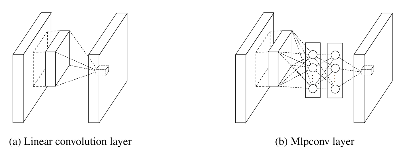
经典的卷积神经网络的结构一般是线性卷积+Pooling + Full Connect, 在这篇文章中，作者认为，在图像识别中要提取的特征常常是非线性的，因此，使用线性的卷积显然无法满足要求。在传统的 CNN 中，为了使用线性卷积去提取非线性特征，常常需要使用大量的线性卷积，这样带来的后果是计算量的大幅增加。NIN 的工作中，为了解决这个问题，作者把线性的卷积改成非线性的卷积。其实，所谓的非线性卷积也是非常简单就能实现：在线性的卷积后面增加一个非线性的映射。

MLP Convolution Layers

如上图 a 是传统的卷积，其表示为 (以 ReLU 为例):

$$ f_{i,j,k}=max\left(w_k^Tx_{i,j},0\right) $$

在 MLP Convolution 中为：

$$ \begin{align} f_{i,j,k_1}^1 &=max\left({w_{k_1}^1}^Tx_{i,j}+b_{k_1}, 0\right) \\ \vdots \vdots\\ f_{i,j,k_n}^1 &=max\left({w_{k_n}^n}^Tf_{i,j}^{n-1}+b_{k_n}, 0\right) \end{align} $$

从上面的数学表达式看上去很复杂，也不好理解，这里给出 caffe 格式网络定义应该更容易理解：

# 前面是正常的卷积操作
# 这里是mlp conv, 可以看出就是一个1*1的卷积操作(等价于全连接操作)
layers {
  bottom: "conv1"
  top: "cccp1"
  name: "cccp1"
  type: CONVOLUTION
  blobs_lr: 1
  blobs_lr: 2
  weight_decay: 1
  weight_decay: 0
  convolution_param {
    num_output: 96
    kernel_size: 1
    stride: 1
    weight_filler {
      type: "gaussian"
      mean: 0
      std: 0.05
    }
    bias_filler {
      type: "constant"
      value: 0
    }
  }
}
# 接着接一个激活函数
layers {
  bottom: "cccp1"
  top: "cccp1"
  name: "relu1"
  type: RELU
}
# 在来一个用1*1的卷积完成的全连接操作
layers {
  bottom: "cccp1"
  top: "cccp2"
  name: "cccp2"
  type: CONVOLUTION
  blobs_lr: 1
  blobs_lr: 2
  weight_decay: 1
  weight_decay: 0
  convolution_param {
    num_output: 96
    kernel_size: 1
    stride: 1
    weight_filler {
      type: "gaussian"
      mean: 0
      std: 0.05
    }
    bias_filler {
      type: "constant"
      value: 0
    }
  }
}
# 接对应的激活函数
layers {
  bottom: "cccp2"
  top: "cccp2"
  name: "relu2"
  type: RELU
}
# 以上完成了两次非线性映射, 也就是 MLP 操作
layers {
  bottom: "cccp2"
  top: "pool0"
  name: "pool0"
  type: POOLING
  pooling_param {
    pool: MAX
    kernel_size: 3
    stride: 2
  }
}
layers {
  bottom: "pool0"
  top: "conv2"
  name: "conv2"
  type: CONVOLUTION
  blobs_lr: 1
  blobs_lr: 2
  weight_decay: 1
  weight_decay: 0
  convolution_param {
    num_output: 256
    pad: 2
    kernel_size: 5
    stride: 1
    weight_filler {
      type: "gaussian"
      mean: 0
      std: 0.05
    }
    bias_filler {
      type: "constant"
      value: 0
    }
  }
}

Global Average Pooling

对于常见的卷积神经网络，我一般把前面的卷积+Pooling 操作看成是一个自动的特征提取器，然后后面的 Full Connect 看做是分类器，最后再接一个 softmax. 然而 Full Connect 由于参数太多，导致两个问题：

容易 overfitting(Drouput 是一种常见的 (标配) 解决这个问题的方法)
参数太多，计算资源需求非常高。

NIN 中提出了 global average pooling 来替代 fc, 所谓 gap 就是最后一层的整个 feature map 上面做 average pooling, 例如，最后一层 conv feature map 是$7 \times 7$, 那么，pooling 的 kernel 大小就是 $7 \times 7$. 这样做的结果是完全不需要训练参数，而且还可以防止 overfitting. 在实践中，需要注意的是把最后一层的 conv kernel 个数设置为输出的类别数就可以了。例如在 ImageNet 中设置为 1000.

layers {
  bottom: "cccp7"
  top: "cccp8"
  name: "cccp8-1024"
  type: CONVOLUTION
  blobs_lr: 1
  blobs_lr: 2
  weight_decay: 1
  weight_decay: 0
  convolution_param {
  # 注意设置最后一个feature map 的输出个数等于类别数
    num_output: 1000
    kernel_size: 1
    stride: 1
    weight_filler {
      type: "gaussian"
      mean: 0
      std: 0.01
    }
    bias_filler {
      type: "constant"
      value: 0
    }
  }
}
layers {
  bottom: "cccp8"
  top: "cccp8"
  name: "relu12"
  type: RELU
}
# Global Average Pooling
layers {
  bottom: "cccp8"
  top: "pool4"
  name: "pool4"
  type: POOLING
  pooling_param {
    # 使用average pooling
    pool: AVE
    # kernel size 等于 feature map 的大小
    kernel_size: 6
    stride: 1
  }
}

Memo

Notes on Network in Network

MLP Convolution Layers

Global Average Pooling